
Language Modeling and Next Token Prediction
The autocomplete on a phone keyboard guesses the next word from the words already typed, and a chatbot that writes whole essays does the same thing many times in a row. A language model is a program that assigns a probability to every possible continuation of a piece of text. A token is one unit of text the model reads and writes, usually a whole word or a piece of one, and the vocabulary is the fixed list of every token the model knows, which holds 32,000 entries in the reference 7B model used across this series. Next token prediction is the task of turning the text so far into a probability for each vocabulary entry being the one that comes next.
Writing, scoring, and training all reduce to that one prediction. Writing repeats it and appends one chosen token each time. Scoring a sentence multiplies the probabilities the model gave to the tokens that really appeared, and training adjusts the model so those probabilities rise. The figure shows the three predictions behind the short sentence “the cat sat”.
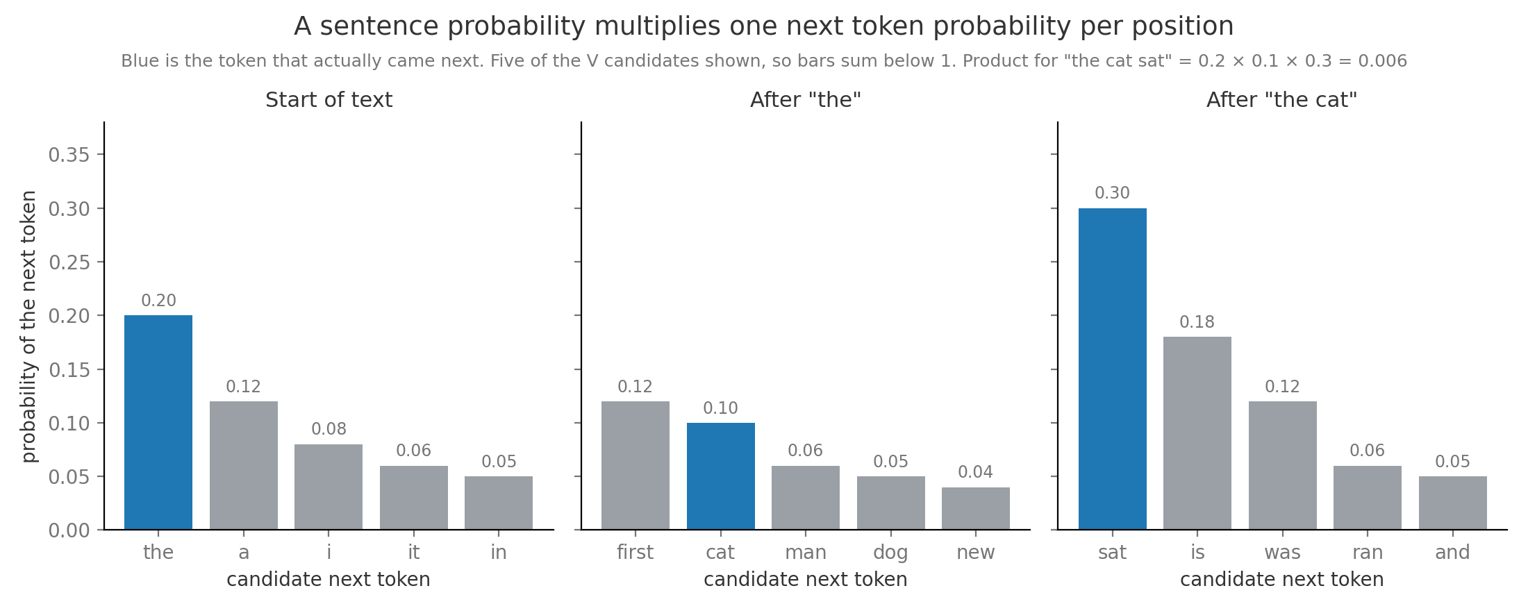
Each panel is a full probability distribution over the vocabulary, but scoring and training read only one bar per panel, the one for the token that actually followed. Everything later in the note, from counting to perplexity, is a different way of producing those panels or of summarizing the bars that were read.
1. Text as a token sequence
Section titled “1. Text as a token sequence”A computer stores text as a list of numbers, and a language model needs a fixed list of units to predict. One could use letters, which gives a tiny vocabulary but very long sequences, or whole words, which gives short sequences but cannot spell a name it has never seen. A tokenizer is the program that cuts raw text into tokens and maps each one to an integer ID between 0 and . Modern tokenizers cut common words into one token and rare words into several pieces, so “the cat sat” becomes three IDs, one per word, while “photosynthesis” is usually cut up. The GPT-2 tokenizer splits it into “photos” and “ynthesis”, and the tokenizer built for BERT, an earlier model for understanding text, splits it into “photos”, “yn”, and “thesis”, which shows that the cuts follow how often letter sequences appear in the training text rather than where the meaningful parts “photo” and “synthesis” meet. A tokenizer with a larger or more science-heavy vocabulary, such as DeepSeek-V3’s, keeps the whole word as one token. How the pieces are chosen is the subject of Tokenization and Embeddings, and this note treats the cut as already made. After tokenization a document is a sequence , where is the token at position and is the length. The prefix is everything before position , and it is all the model is allowed to see when predicting . Under the hood text is also stored as bytes, the 8-bit units a file is made of, with one byte per ordinary English letter in the common UTF-8 encoding. We will come back to bytes in section 8, since every tokenizer agrees on how many bytes a text has, which makes them a fair unit for comparing models. The reference 7B model reads up to 4,096 tokens at once and chooses from 32,000 vocabulary entries at every position. A 4,096-token document therefore poses 4,095 separate prediction problems, each with 32,000 possible answers, and pretraining on 2 trillion tokens poses about 2 trillion of them.
2. The chain rule of probability
Section titled “2. The chain rule of probability”Guessing a whole sentence at once is hopeless, since even short sentences are almost all unique, but guessing one word given the words before it is manageable. A conditional probability is the probability of one event once you already know another has happened, written and read “the probability of A given B”. The chain rule of probability says the probability of several events together equals the probability of the first, times the probability of the second given the first, and so on. For text it splits one impossible question into manageable ones:
Here means multiply the factors for through , is the token at position , is the prefix before it, and is the model with parameters . The first factor conditions on an empty prefix, meaning the start of the text. The equation is exact rather than an approximation, so a model that gets every next-token probability right gets every sentence probability right. A model that generates this way, one token at a time with each new token conditioned on all earlier ones, is called autoregressive.
Take the three predictions in the opening figure. The model gave “the” probability 0.2 at the start, “cat” probability 0.1 after “the”, and “sat” probability 0.3 after “the cat”. The sentence probability is . Multiplying many small numbers creates a practical problem. If every token of a 1,000-token document had probability 0.1, the document’s probability would be , far below the smallest positive number a 32-bit float, the usual format a computer uses for a decimal number, can hold, which is about , so the computer would store exactly zero and every long document would look equally impossible. Working with logarithms avoids this, because the log of a tiny probability is an ordinary negative number, such as . The log probability, the natural logarithm of a probability, turns the product into a sum: , and recovers the product. Every practical system adds log probabilities, and the loss in section 6 is the same sum with its sign flipped.
3. Counting models and smoothing
Section titled “3. Counting models and smoothing”The simplest way to estimate how likely “sat” is after “the cat” is to look through a large pile of text and count. A corpus is the collection of text a model learns from. An n-gram is a run of consecutive tokens, so “the cat” is a 2-gram, or bigram, and “the cat sat” is a 3-gram, or trigram. Classical systems such as the trigram models behind 1990s speech recognizers predicted the next word from counts alone. The Markov assumption makes counting possible by keeping only the last tokens of the prefix and forgetting the rest, so a bigram model predicts from one previous token. The maximum likelihood estimate for a bigram model is then a ratio of counts:
Here counts how often the pair occurs in the corpus and counts how often the first token occurs. Take the twelve-token corpus “the cat sat . the dog sat . the cat ran .” where the period counts as a token. “the” occurs 3 times and “the cat” twice, so . “dog” occurs once and is followed by “sat”, so and . That zero is the central failure of counting. The zero count problem is that any sequence missing from the corpus gets probability exactly zero, and by the chain rule one zero factor makes the whole sentence probability zero and its log probability minus infinity. “the dog ran” is a perfectly ordinary sentence, but this model calls it impossible because “dog ran” never appeared. Sparsity, the fact that most possible n-grams never appear in any finite corpus, makes the zero count problem the normal case once reaches three. The figure measures this on real text, about 1.8 million words of the author’s study notes, with a tenth of the files held back as a test.
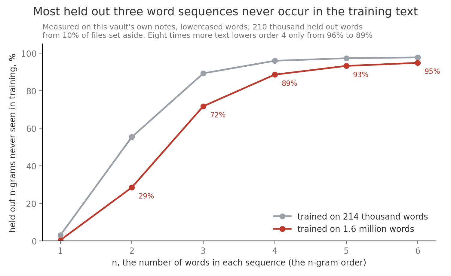
On that text 72% of held-back three-word sequences never occur in the 1.6 million training words, and eight times more training text barely helps at four words and beyond. At the scale of the reference 7B model the arithmetic is starker. With there are possible trigrams, and a 2-trillion-token corpus contains at most trigram occurrences, so at most 6.1% of possible trigrams could ever be seen even once. Possible 4-grams number about .
Smoothing on a toy corpus
Section titled “Smoothing on a toy corpus”Smoothing is any rule that moves a little probability from sequences that were seen to sequences that were not, so nothing gets exactly zero. Add-one smoothing, also called Laplace smoothing, pretends every possible pair occurred once more than it did, which gives . Backoff keeps the observed counts but shaves a discount off each one, then hands the freed probability to unseen continuations in proportion to how common each token is on its own. The table works both after the context “dog” in the twelve-token corpus, where the toy vocabulary has tokens, the context count is , and the discount is . On its own, “the” occurs 3 times, “cat” 2, “sat” 2, “dog” 1, “ran” 1, and the period 3, out of 12 tokens.
| Next token | Count after “dog” | Raw counting | Add-one | Backoff with |
|---|---|---|---|---|
| sat | 1 | 1.000 | 2/7 = 0.286 | (1 − 0.5)/1 = 0.500 |
| ran | 0 | 0 | 1/7 = 0.143 | 0.5 × 1/10 = 0.050 |
| the | 0 | 0 | 0.143 | 0.5 × 3/10 = 0.150 |
| cat | 0 | 0 | 0.143 | 0.5 × 2/10 = 0.100 |
| dog | 0 | 0 | 0.143 | 0.5 × 1/10 = 0.050 |
| . | 0 | 0 | 0.143 | 0.5 × 3/10 = 0.150 |
Both columns sum to one and both rescue “dog ran”. Add-one does it bluntly, cutting the one thing the corpus actually showed from 1.0 to 0.286, and with a realistic vocabulary of 32,000 the invented counts would swamp any real ones. Backoff keeps “sat” at 0.5 and spreads the freed half by how common each token is, which is why every serious counting model, up to Kneser-Ney smoothing developed in Language Models before Transformers, is a refinement of discounting and backoff. Neither rule knows that a dog is like a cat, and that missing knowledge is what the next section supplies.
4. Neural language models
Section titled “4. Neural language models”A person who has read “the cat ran” but never “the dog ran” still finds the second sentence unsurprising, because cats and dogs behave alike. A counting model has no notion that two words are alike, since every n-gram is a separate entry in a table. A neural network is a function built from many simple arithmetic steps whose behavior is set by adjustable numbers called parameters, and a neural language model uses one to compute next-token probabilities instead of looking them up. Bengio and colleagues introduced the design in 2003, and every modern large language model, or LLM, keeps its three stages.
- An embedding is a learned vector of numbers stored for each vocabulary token, and the model starts by looking up for every token in the prefix. The reference 7B model stores such numbers in its embedding table. How the lookup works and what the vectors learn is covered in Tokenization and Embeddings.
- The network body combines the prefix embeddings into one hidden state , a vector of numbers summarizing everything the prefix says about what comes next. In modern models the body is a stack of transformer layers, blocks that let each position read the earlier positions and then transform what it read, as described in The Transformer Block and Model Anatomy.
- An output head stores one output vector per vocabulary token and scores each candidate by the dot product , which multiplies matching entries and adds them up. In the reference 7B model the output head is a second, untied table of another 131,072,000 numbers.
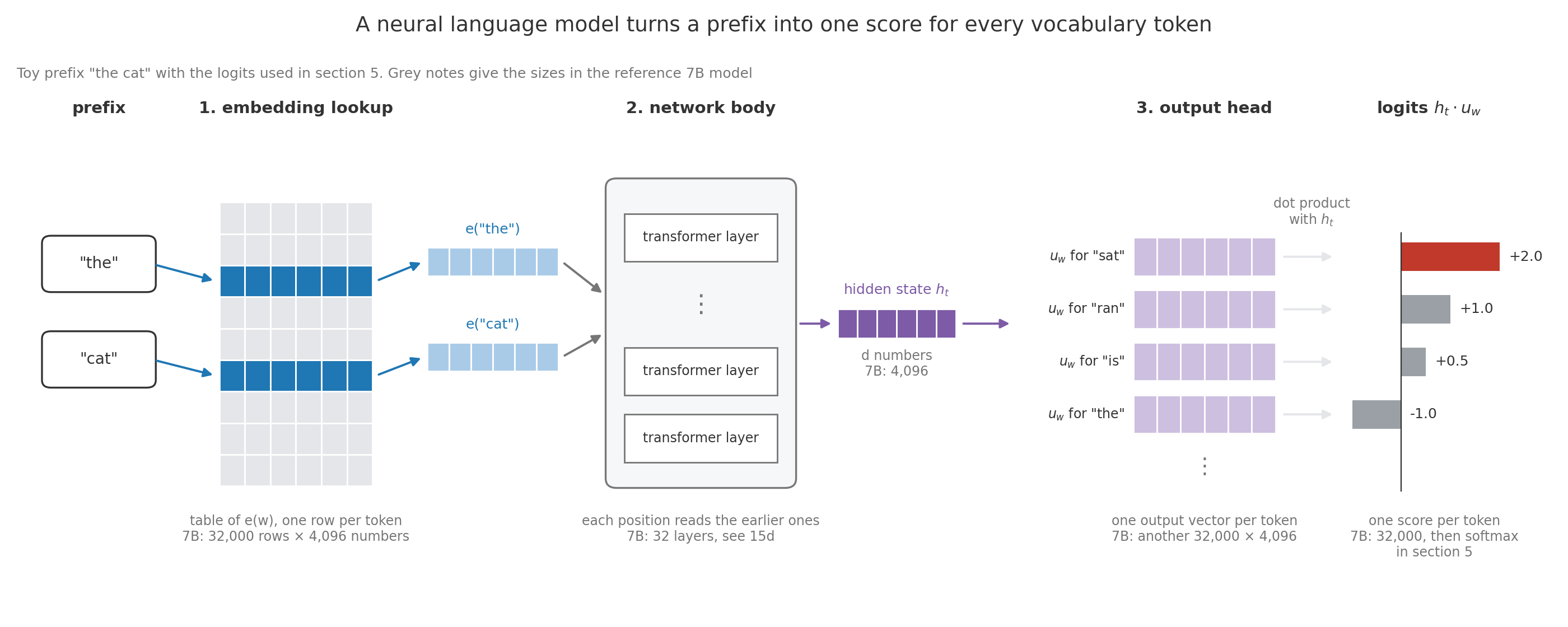
The figure follows the prefix “the cat” through the three stages. Two rows are read out of the embedding table, the network body mixes them into one hidden state, and that state is scored against every output vector, giving the logits that section 5 turns into probabilities.
Training means adjusting the parameters so the model gives higher probability to the tokens that really came next in the corpus. It runs by gradient descent, which repeatedly nudges every parameter a small step in the direction that most increases those probabilities. Section 6 names the exact quantity being pushed. The gain over counting comes from where the knowledge is stored. Take a toy model with in which the hidden state is just the embedding of the previous token. Suppose training has placed and close together, because both appear before “sat”, “ate”, and “barked” in many sentences, while sits elsewhere. With , the score for “ran” after “cat” is , after “dog” it is , and after “the” it is .
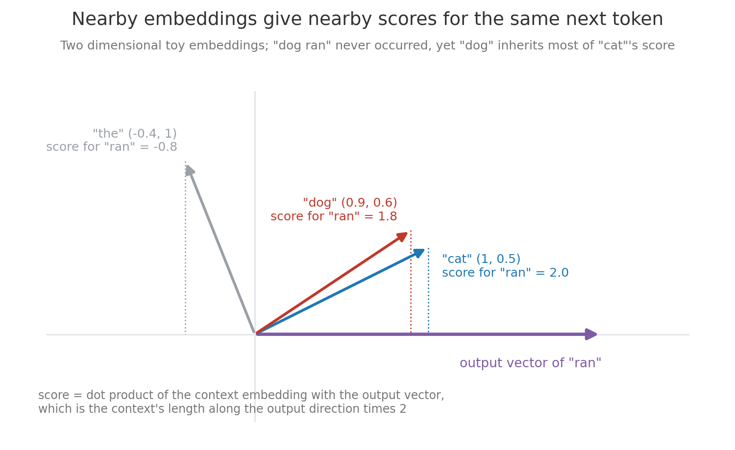
Every time training raised the score of “ran” after “cat”, it moved toward , and that same move raised the score after “dog” because the two embeddings are neighbors. Statisticians call this sharing statistical strength, meaning evidence about one context improves predictions for every similar context. That is how the model gives “dog ran” a sensible probability with no count at all. It also means the model needs no table entry per n-gram, so the parameter count stays fixed as the prefix grows from 2 tokens to 4,096.
5. Logits and softmax
Section titled “5. Logits and softmax”The scores from the output head can be any real numbers, such as 2.0 or −1.0, but a probability must be between 0 and 1 and the probabilities over all candidates must sum to 1. A logit is the raw score for candidate before that conversion. Softmax is the function that does the conversion. It raises , about 2.718, to the power of each logit, which makes every value positive while keeping the larger logit larger, and then divides each result by their sum:
Here is the logit for candidate , the sum runs over every vocabulary token , and is the temperature defined below, equal to 1 during training and scoring. Take the context “the cat” with four candidates whose logits are 2.0 for “sat”, 1.0 for “ran”, 0.5 for “is”, and −1.0 for “the”. The exponentials are 7.389, 2.718, 1.649, and 0.368, their sum is 12.124, and dividing gives 0.609, 0.224, 0.136, and 0.030. Only the gaps between logits matter, since adding the same number to every logit multiplies every exponential by the same factor, which cancels in the division. Real code uses that fact to keep softmax numerically stable. It subtracts the largest logit before exponentiating, and when only the log probability is needed, as in the loss of section 6, it computes that log directly:
Here is the largest logit and . Every exponent is now zero or below, so no exponential exceeds 1 and the largest one equals exactly 1, which keeps the sum away from both overflow and zero. Logits of 1,000 and 999, whose exponentials overflow to infinity, become 0 and −1 and give the same weights of 0.731 and 0.269. The second form is called log-sum-exp, and it never takes the log of a probability that may have rounded to zero. Implementations also do this sum in 32-bit precision even when the rest of the model runs in a smaller format.
Temperature is a positive number that divides every logit before softmax. Dividing by 0.5 doubles every gap, and the same four candidates become 0.842, 0.114, 0.042, and 0.002, so the top choice dominates. Dividing by 2 halves every gap and flattens them to 0.434, 0.263, 0.205, and 0.097. Sampling means drawing the next token at random according to these probabilities, and temperature is the simplest control over how adventurous sampling is. Decoding rules built on it, such as top-p sampling, belong to Inference and Decoding, and every loss and perplexity in this note assumes .
The animation replays the calculation column by column, shows that subtracting the largest logit changes nothing, and then redraws the bars at temperatures 0.5 and 2 over dashed outlines of the temperature 1 answer.
6. Cross entropy loss
Section titled “6. Cross entropy loss”Training needs one number that says how badly the model did on a token, so that gradient descent has something to push down. A loss function is that number, chosen so a perfect prediction scores zero and worse predictions score higher. Language models use the negative log likelihood, or NLL, which for one token is minus the log of the probability the model gave to the token that actually came next, averaged over the scored tokens:
Here is the number of tokens scored, is the true token at position , and is the true prefix before it. The minus sign makes the loss positive, since the log of a number below one is negative, and dividing by makes it an average per token. With natural logs the unit is the nat. With base-2 logs the unit is the bit, the surprise of one fair coin flip, and one bit equals nats, so dividing nats by 0.693 converts them to bits.
Papers usually call the same number cross entropy. In general, cross entropy compares a target distribution with the predicted one at every scored position and averages over the positions:
Here the inner sum runs over every vocabulary token , and is the target weight on token at position , written when the position is clear. In next-token training the target is one-hot, meaning weight 1 on the token that actually came next and 0 on every other token, so the inner sum keeps only the true token’s term, , and becomes exactly the NLL formula above. The two names part only when the target spreads over several tokens, as in distillation from a teacher model’s probabilities in Post Training from Base Model to Assistant.
Why use NLL
Section titled “Why use NLL”NLL is not the only possible loss. Any formula that gets smaller as the model gives the true token more probability could, in principle, be used for training, such as , where is the probability given to the true token, or a squared error. Take the prefix “The capital of France is” with “Paris” at 0.80, “London” at 0.10, “Berlin” at 0.06 and “Rome” at 0.04. NLL charges nats for “Paris”, and it would charge 0.01 at , 0.69 at , and 4.61 at . Language models use NLL rather than these other losses because of the following five strengths.
- It is maximum likelihood. By the chain rule of section 2 a text’s probability is a product of next-token probabilities, and the log turns that product into a sum, so the summed NLL over a text is exactly minus the log probability of the whole text, . For “the cat sat” that is nats, the same total as from the per-token losses in the worked example above. Lowering it raises the probability of the training data, which is the estimation rule section 9 develops, and because the sum has one term per token, a batch of tokens is scored by averaging their terms.
- It keeps numbers in range. A 4,096-token window whose true tokens average probability 0.2 has probability , far below the smallest positive 32-bit floating-point number, about , so the product rounds to zero. Its log is nats, an ordinary number.
- Its push does not fade when the model is badly wrong. The gradient of the loss is the list of how much it changes when each input moves a little, and through softmax the gradient of NLL with respect to each logit is . For the four candidates in section 5 with “sat” true that is , so gradient descent raises the true token’s logit and lowers each other logit in proportion to the probability it wrongly received. With as the loss, the true logit’s gradient is instead, so at NLL pushes with while pushes with , a hundred times weaker exactly when the model most needs correcting.
- It trains faster than squared error. The squared distance between the predicted probabilities and the one-hot target, called the Brier score, , is a legitimate loss, but through softmax its gradient also shrinks when the model is confidently wrong. Suppose all the remaining probability sits on one wrong token. Then the score is , which is only 1.96 at , compared with an NLL of 4.61. The push on the true token’s logit is , which is at , twenty-five times weaker than NLL’s . NLL also grows without bound as falls, so a model can never safely call an observed token impossible.
- It rewards honest uncertainty. NLL is a proper scoring rule, meaning its average over the data is lowest when the predicted distribution equals the true one, as section 9 shows. After “She went to the store to buy some”, where “milk”, “bread” and “fruit” all occur, the best NLL comes from giving each its real frequency rather than betting everything on one. The Brier score shares this property, but does not, since its average is lowest when all probability sits on the single most common token.
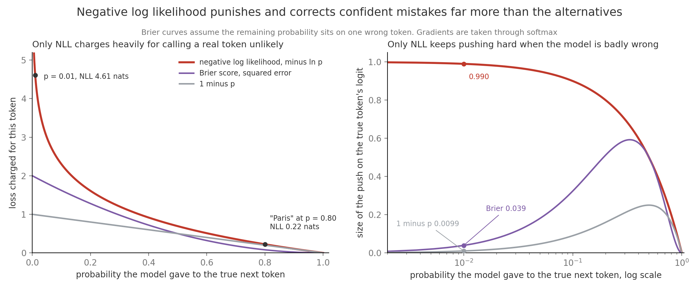
The left panel shows the penalty each rule charges, and only NLL climbs steeply on the left, where cutting a probability in half always adds exactly one bit. The right panel shows how hard each rule pushes the true token’s logit, and only NLL keeps pushing near full strength as approaches zero. That shape forces a model trained on NLL to keep some probability on everything that occurs in the data, which section 9 turns into a statement about the whole distribution. NLL also has an important limit. It measures how well the model predicts its training text, not whether an answer is true, well reasoned, or what a person wanted, which is why the post-training in Post Training from Base Model to Assistant adds objectives built on preferences and checked answers.
7. Perplexity
Section titled “7. Perplexity”Section 6 gave “the cat sat” an average loss of 1.705 nats per token. The number is correct, but few people have a feel for what 1.705 nats means. A count of choices is much easier to picture, and the two are directly linked. Suppose a model has to guess the roll of a fair six-sided die. The best it can do is give each face probability 1/6, so every guess costs nats. The same reasoning works for any number of options. With equally likely options, each one gets probability , so each guess costs nats. That gives a way back from a loss to a number of options: the loss is , so raising to the loss undoes the log and recovers . For the die, , which is the six faces we started with. Perplexity applies that conversion to any model. It takes the model’s average loss and returns the number of equally likely options that would give the same loss:
Here is the average cross entropy in nats from section 6, and the second form shows that perplexity is the geometric mean, the -th root of a product of numbers, of one over each true-token probability. Perplexity is therefore read as an effective branching factor, the number of equally likely next tokens the model was effectively choosing between at each step. If losses are in bits, the same number is . For “the cat sat”, , and the second form agrees, since . The model was as uncertain as someone picking uniformly among about five and a half tokens. A model that spreads probability evenly over the whole vocabulary gives every token , so its loss is and its perplexity is exactly . For the reference 7B model that is nats and a perplexity of 32,000, and a freshly initialized model whose first logged loss sits far above 10.37 usually has a bug in its initialization or in how the loss is averaged. A loss of 2.3 nats gives , the uncertainty of a fair ten-sided die. Perplexity is always measured on held out text, meaning text kept out of training, since a model can memorize its training text and look better than it is.
The animation builds the running total and running average one token at a time, exponentiates the average, and ends on the uniform-model comparison. Because perplexity is an exponential, equal drops in loss give unequal drops in perplexity. Going from 2.3 to 2.2 nats takes perplexity from 10.0 to 9.0, while going from 1.1 to 1.0 takes it from 3.0 to 2.7.
Perplexity is the standard way to report a language model’s loss because it helps in four practical ways.
- It makes progress readable. Saying a new checkpoint cut the model’s choice from about 10 equally likely tokens to about 9 is easier to judge than saying its loss fell from 2.3 to 2.2 nats, so training curves and model reports usually show perplexity.
- It gives quick sanity checks. A fresh model should start near a perplexity of , 32,000 for the reference model, and a model scoring near 1.5 on new general text is almost certainly being tested on text it has already seen, because no model is that sure of ordinary writing.
- It shows how well a model fits a kind of text. Measuring perplexity on held out legal, medical, or code documents tells you how familiar the model is with that domain’s language before you spend money adapting it, and a drop after extra training on that domain shows the training worked.
- It can score data as well as models. Pipelines such as CCNet run a small language model over web pages and keep the ones whose perplexity looks like clean reference text, which removes spam and broken pages before pretraining.
Perplexity has two limits. Two models can only be compared on the same held out text with the same tokenizer, which section 8 fixes with bits per byte. And a lower perplexity says the model predicts text better, not that it answers questions better, which is why 15i measures task quality separately.
8. Bits per byte across tokenizers
Section titled “8. Bits per byte across tokenizers”Comparing models is one of the most common reasons to measure loss, for example when choosing between two open models or checking whether a new tokenizer helped, and the models being compared often use different tokenizers. That is a problem for perplexity, because perplexity is an average per token and two tokenizers cut the same text into different numbers of tokens. A fine tokenizer that splits words into small pieces makes many easy predictions, such as finishing a word whose first half is already written, and those easy predictions pull the per-token average down without the model being any better. Bits per byte, or BPB, divides the total loss by the number of bytes in the raw text instead of the number of tokens, so it charges every model for the same text regardless of how it was cut:
Here the numerator is the total loss over all tokens in bits, is the byte count of the text, is the average loss in nats per token, and dividing by converts nats to bits. The Pile reports its language model results this way for exactly this reason. Score the 22-byte sentence “the cat sat on the mat” with two models. Model A uses a coarse tokenizer that produces 6 tokens and pays 12.0 nats in total. Model B uses a fine tokenizer that produces 9 tokens and pays 12.6 nats. Per token, A averages 2.0 nats and a perplexity of , while B averages 1.4 nats and a perplexity of , so B looks far better. Per byte, A pays bits and B pays bits, so A is actually better, since it paid less to encode the same sentence.
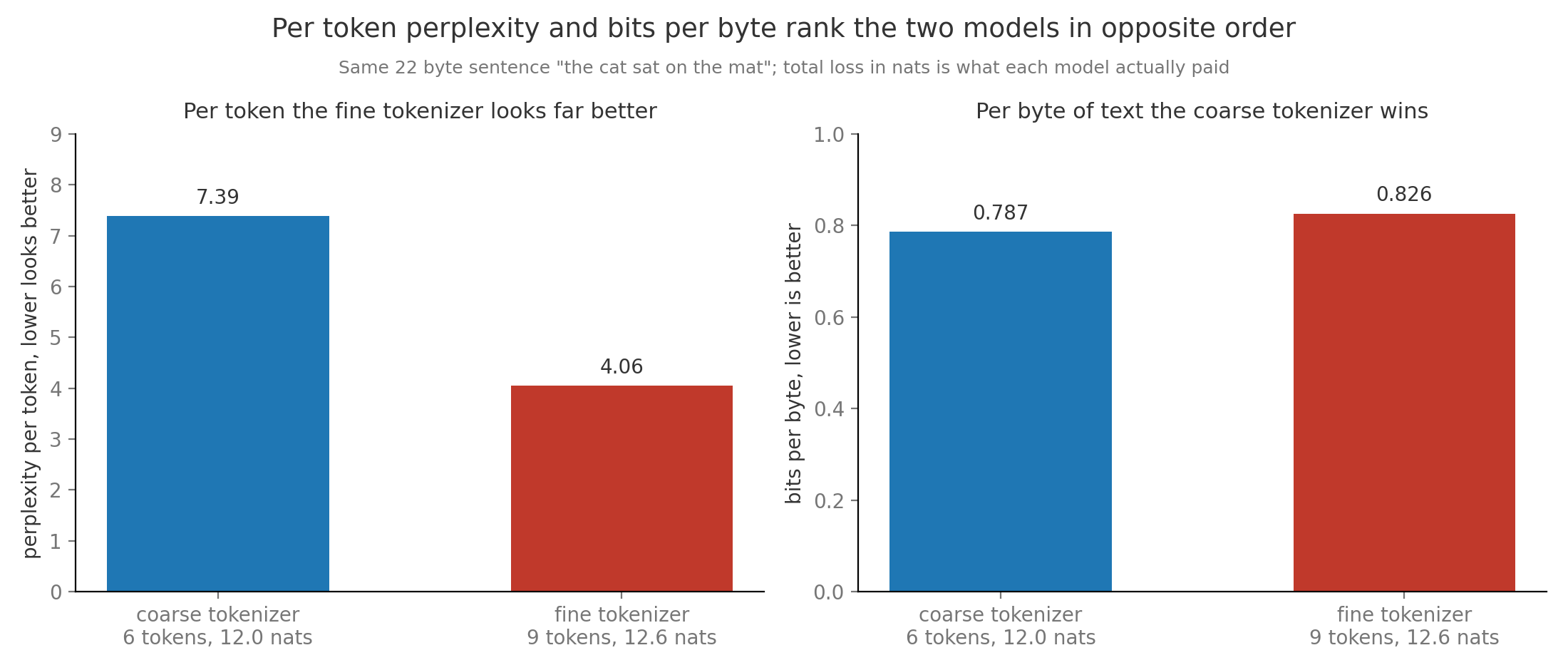
At the scale of the reference 7B model, suppose it reaches a held-out loss of 1.8 nats per token on English text and its 32,000-token vocabulary averages roughly 4 bytes per token. That is a perplexity of , or bits per byte. A model with a 128,000-token vocabulary at 5 bytes per token would report a higher per-token loss on the same text even if it compressed the text better, so the comparison has to be done in bits per byte.
9. Maximum likelihood as distribution matching
Section titled “9. Maximum likelihood as distribution matching”Section 6 trains a model by lowering the average loss on observed tokens, which raises the probability of the data, but it is not obvious that this makes the model’s whole distribution resemble real text. That question matters for two reasons. A model is used by sampling from its whole distribution, so a model that ranks the right token first but gets the other probabilities wrong will still write odd text. And knowing how much of the loss could still be removed tells you whether more training or a bigger model is worth paying for. The data distribution is the unknown process that produced the corpus, and each corpus sentence is one draw from it. Maximum likelihood is the training rule of choosing the parameters that make the observed data most probable, which is the same as minimizing cross entropy on it. Seen at one prefix, the average loss over many draws is the cross entropy between two distributions, and it splits into two parts.
The last term, the Kullback-Leibler divergence explained just below, is computed as
Here is the expected loss when the truth is and the model predicts with . Entropy is the loss of a model that knows the truth exactly, the irreducible uncertainty of language itself. Kullback-Leibler divergence, or KL divergence, is the extra loss paid for using the wrong distribution, which is zero only when the two match. The entropy does not depend on , so minimizing cross entropy is the same as minimizing KL divergence from the data to the model. The split also answers the second question above. Entropy is a floor that no model can go below, so only the KL divergence part of a loss is room for improvement.
Take a prefix where the true next-token distribution over three tokens is . Its entropy is 1.030 nats, the best loss any model can reach. A model predicting has cross entropy 1.122 nats, so its KL divergence is . The definition gives the same number directly, since . An overconfident model predicting has cross entropy 2.313 nats and a KL divergence of 1.283, fourteen times worse, even though it puts the most likely token first. It loses because it gave 0.01 to tokens the data produces 30% and 20% of the time. That asymmetry gives maximum likelihood its character. Mode covering is the tendency to put probability everywhere the data goes, even at the cost of also putting some where the data never goes, because missing real data costs far more than wasting probability. The opposite direction, , is mode seeking, which prefers to fit one region of the data well and ignore the rest. Reinforcement learning from human feedback, covered in Post Training from Base Model to Assistant, behaves more like the second, which is one reason assistants sound narrower and more certain than base models.
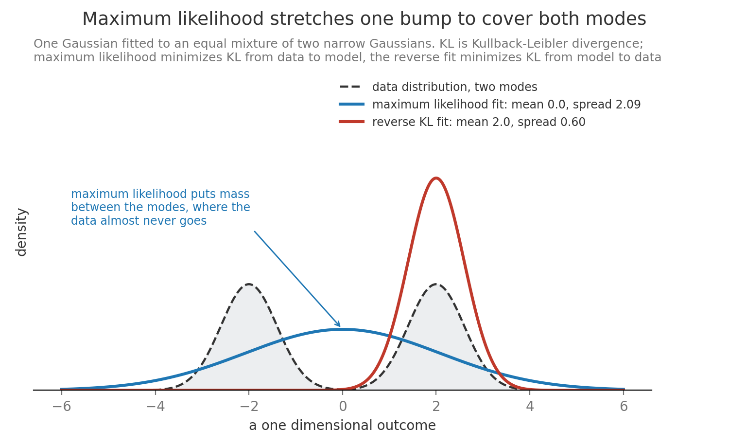
The figure fits one bell curve to data with two separate peaks. The maximum likelihood fit sits between the peaks and spreads wide enough to cover both, while the reverse fit locks onto one peak. For text, the covering behavior is why a pretrained model, sampled at temperature 1, sometimes produces strange continuations it has learned are merely possible.
10. Teacher forcing and exposure bias
Section titled “10. Teacher forcing and exposure bias”A student practicing translation with an answer key checks each word against the key and then continues from the key’s version, even when their own word was wrong. Teacher forcing trains a language model the same way. At every position the model predicts from the true prefix in the corpus, never from its own earlier guesses, so the loss for “sat” is computed after the true “the cat” even if the model would have written “the dog”. This lets all positions of a sequence be scored in one parallel pass, since every prefix is already known, so one 4,096-token sequence in the reference 7B model yields 4,095 training predictions at once. Teacher forcing is how large language models are actually trained during pretraining and during supervised fine-tuning, the later stage that trains on example answers, and this parallel scoring is the main reason, since generating one token at a time during training would be far too slow over trillions of tokens. Generation works differently. Free-running generation feeds each sampled token back in as part of the prefix, so after the first mistake the model is conditioning on text that came from itself rather than from the corpus. This is how a model writes when people use it, and it is also how the model produces its own training examples during reinforcement learning in post-training, the one training stage that learns from free-running output instead of the true prefix.
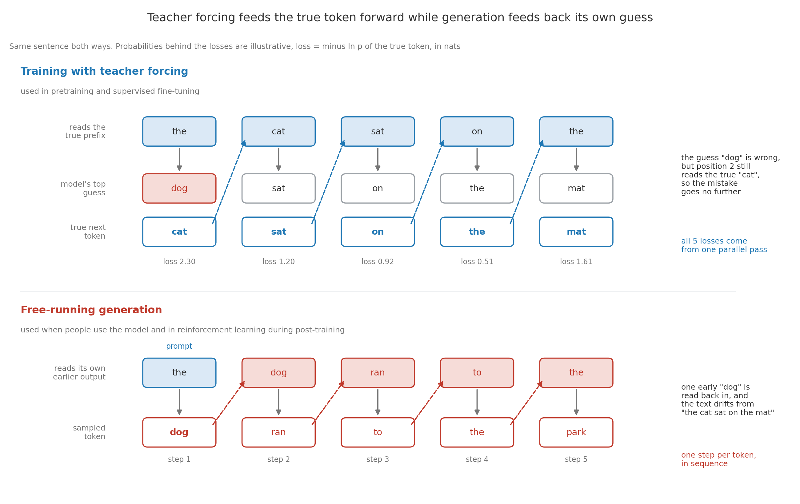
The figure runs both methods on “the cat sat on the mat”. Under teacher forcing, the model’s top guess after “the” is the wrong word “dog”. That costs 2.30 nats, because the true “cat” got only probability 0.10. Position 2 still reads the true “cat”, though, so the mistake goes no further, and all five losses come from one pass. Under generation, the same early “dog” is fed back in. Every later step builds on it, and the text becomes “the dog ran to the park”.
Exposure bias is the mismatch teacher forcing creates, since the model was never trained on prefixes containing its own errors and may not know how to recover from them. If each token had an independent 1% chance of an unrecoverable slip, a 500-token answer would come out clean with probability . Scheduled sampling (Bengio and colleagues, 2015) addressed it by gradually replacing true prefix tokens with the model’s own samples during training. Large modern models mostly do not use scheduled sampling, partly because feeding in the model’s own samples breaks the single parallel pass, and the pessimistic calculation overstates the problem for them. Their pretraining text already contains typos, digressions, and corrections, so recovering from an odd prefix is partly learned, and most slips are not unrecoverable. The concern has not vanished, though, since repetition loops under greedy decoding, studied by Holtzman and colleagues, and drift over very long reasoning traces are both symptoms of a model feeding on its own output. The stage of LLM training that does not use teacher forcing is reinforcement learning during post-training, with methods such as Proximal Policy Optimization (PPO) and Group Relative Policy Optimization (GRPO), covered in Post Training from Base Model to Assistant. There the model writes complete answers itself, the answers are scored, and the update is computed on those self-generated prefixes, which directly reduces the exposure-bias gap.