
The Transformer Block and Model Anatomy
A large language model is one repeated unit stacked many times, and that unit explains most of the model’s size, cost, and training behavior. The model holds each token, a word or piece of a word, as a list of numbers, and a stack of identical units called blocks reads that list and adds a correction to it rather than rewriting it. A transformer is a neural network built from such blocks, and a neural network is a learned numerical function whose adjustable numbers are its parameters. Most questions about model size, training cost, and stability come down to how those blocks are wired, which is separate from what the model is trained to predict.
Each block holds two parts, and both follow the same routine. Attention lets a token pull information from earlier tokens, and the feed-forward network transforms each token on its own. Each part reads a rescaled copy of the running list, computes something, and adds the result back. Once that routine is clear, the model’s anatomy reduces to counting. Count the matrices to get the parameters, multiply by two to get the arithmetic per token, and swap one part for several copies to get a mixture of experts.
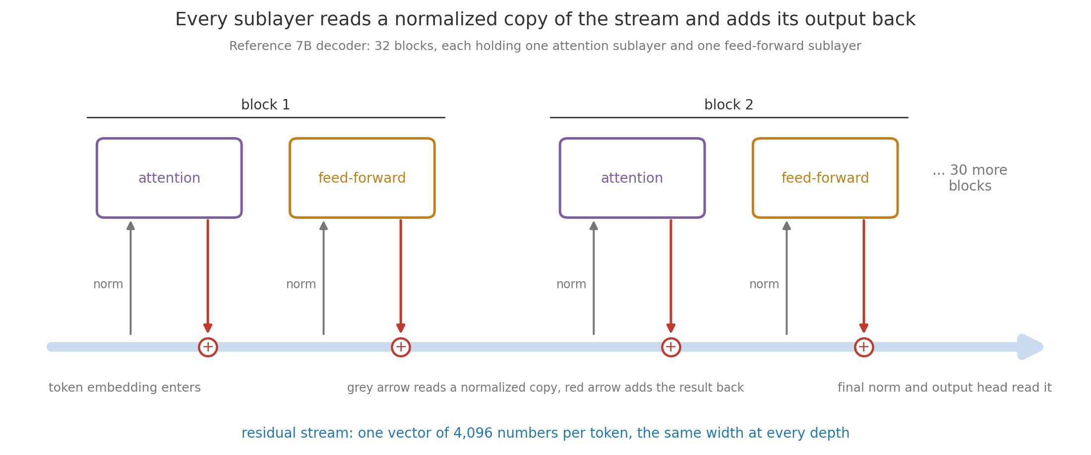
The figure carries the main idea of the whole note. The stream keeps the same width from the embedding at the bottom to the output head at the top, and no block ever overwrites it. Because the blocks only add, the final vector is the embedding plus 64 sublayer contributions, and a gradient can reach any block straight down the identity path.
1. The residual stream
Section titled “1. The residual stream”Any deep stack has to answer one design question, which is whether each layer replaces its input or edits it. Think of a document passed around a team. If each person retypes the whole thing from memory, mistakes compound and the early content fades, while tracked edits keep the original and add each change on top. A residual connection is that tracked-edit design: a layer’s output is added to its input instead of replacing it. The residual stream is the running vector those additions build up, one per token, from the embedding (the learned starting vector looked up for the token, covered in Tokenization and Embeddings) to the final layer. It was introduced for image networks by ResNet and is used in every transformer since the original Transformer.
Each block contains two sublayers, attention and then the feed-forward network. Treating a whole block as one update for now, block changes the stream by , where is the stream entering, is what block computes from it, and is the stream leaving. Section 6 shows that a block actually makes this addition twice, once per sublayer. Unrolling the sum over all blocks gives , with each evaluated on the stream it read, so the final vector is literally the embedding plus every contribution.
Three blocks on a two-number stream
Section titled “Three blocks on a two-number stream”The steps below run a two-number residual stream through three blocks. They show that the final vector is simply the starting embedding plus each block’s addition, so removing one block removes exactly its contribution.
- Start with an embedding of . Real streams have 4,096 numbers, but two are enough to draw.
- Block 1 computes from what it read and adds it, giving .
- Block 2 adds , giving , and block 3 adds , giving the final stream .
- Zero out block 2 and the final vector becomes . It moves by exactly block 2’s contribution, because the blocks’ writes are added rather than chained.
The animation replays steps 1 to 4. The same additive structure is what keeps training possible at depth. The loss is a single number measuring how wrong the model’s predictions are. A gradient is the signal saying how much the loss would change if a parameter moved, and training sends it backward from the output through every layer. In a plain stack each layer multiplies the gradient by its own local slope, so 32 layers that each scale it by 0.5 shrink it to , which is the vanishing gradient problem. With residual connections the derivative of with respect to any always contains a term equal to 1 from the identity path, so block 1 receives the top-level gradient undiminished plus whatever the blocks above add to it. Interpretability work often reads the stream as a shared workspace that attention moves information into and the feed-forward network writes facts into, a view developed in Anthropic’s transformer circuits framework.
2. Layer normalization and RMSNorm
Section titled “2. Layer normalization and RMSNorm”Adding contributions block after block lets the stream’s numbers drift in size, and a sublayer that sees inputs ten times larger than last week will behave differently. Exam scores have the same problem across classes, and converting each class to standardized scores makes them comparable. Normalization is that rescaling step: it takes a vector and returns a version with a standard size, so the next layer always sees inputs on a predictable scale. Layer normalization, or LayerNorm, from Ba et al., works within one token’s vector. It subtracts the mean of the coordinates, divides by their standard deviation, then applies a learned scale and shift:
Here is the average of the coordinates, is their standard deviation, is a tiny constant such as that keeps the denominator above zero, and multiplies coordinate by coordinate. The gain is a learned scale per coordinate and the offset is a learned shift per coordinate, which together let the model undo the standardization where that helps.
RMSNorm, from Zhang and Sennrich, skips the mean subtraction and the offset, and divides by the root mean square instead, the square root of the average squared coordinate , and then multiplies by the same learned gain :
One vector normalized both ways
Section titled “One vector normalized both ways”The steps below normalize the same four-number vector with LayerNorm and with RMSNorm, so you can see exactly what RMSNorm leaves out.
- Take with gain 1 and no offset, and ignore .
- LayerNorm first finds the mean, . The deviations are , their squares average to , and the standard deviation is . Dividing the deviations gives the LayerNorm output , whose mean is 0 and whose standard deviation is 1.
- RMSNorm instead averages the raw squares, , so , and dividing gives . The signs and the positive mean survive, and only the overall size is standardized.
- A learned gain of would then double the last coordinate, giving .
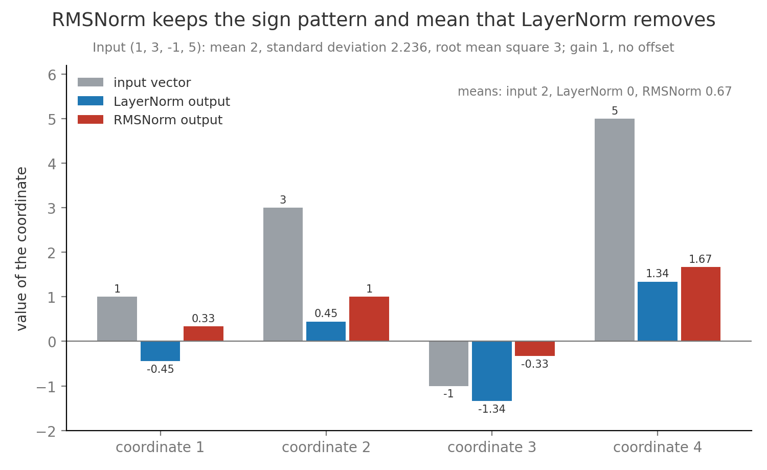
RMSNorm saves the mean computation and the offset numbers, and the paper reports 7% to 64% faster normalization with matching quality. Its argument is that rescaling to a fixed size, which both methods do, carries the stabilizing benefit, while recentering adds little. Llama, Mistral, and most recent decoders use it. In the reference 7B each RMSNorm holds 4,096 gain numbers, two per block plus one final, which is 266,240 parameters in total.
3. Pre-norm and post-norm placement
Section titled “3. Pre-norm and post-norm placement”Once a block has a normalization step, the remaining question is where to put it, either on the way into each sublayer or after the addition. A kitchen that checks every ingredient before it goes into the pot is checking inputs, while one that checks the soup after every addition is checking the running result. Post-norm, used in the original Transformer, normalizes after the addition, . Pre-norm, used from GPT-2 onward, normalizes only the copy the sublayer reads, , and leaves the stream itself untouched. In both, is the stream entering, is the sublayer’s computation, and Norm is LayerNorm or RMSNorm.
The difference is what happens to the identity path from section 1. In post-norm every normalization sits on that path, so a gradient travelling from the top to block 1 passes through 64 rescalings, and Xiong et al. showed that at the start of training the gradients near the output are much larger than those near the input. Post-norm stacks therefore need warmup, a schedule that starts the step size near zero and raises it over the first few thousand steps, and deep post-norm stacks still diverge easily. Pre-norm keeps the identity path free of any operation, so the 1 from section 1 reaches every block, and deep stacks usually train without warmup tricks. Pre-norm has its own cost. The stream is never rescaled, so it grows. If the embedding has a root mean square of 1 and each of 32 blocks adds a contribution of size 1 that is roughly unrelated to the others, the squared sizes add and the final stream has size about . A late block’s write then changes the stream’s direction by about one part in 5.7, which is one reason late layers in pre-norm models often contribute less, and it is why a final normalization before the output head is mandatory. Some recipes add extra norms or rescale the residual branches to recover late-layer influence, and those are refinements on a pre-norm base.
4. The feed-forward network
Section titled “4. The feed-forward network”Attention mixes information across tokens, but something also has to compute on what each token has gathered. A recipe card that has collected ingredients from several shelves still needs a cooking step that turns them into a dish. The feed-forward network, or FFN, is that step: a small two-layer network applied to each token’s vector separately, with the same weights for every position. It widens the vector, applies a nonlinear function to each number, and narrows it back:
Here is the normalized stream for one token as a row of numbers, is a matrix that widens it, is the activation function applied to every number separately, and is a matrix that narrows it back. The hidden width is the number of hidden units, classically . A matrix of shape holds parameters, so the classic FFN holds , which at is 134,217,728, twice the of attention. Two thirds of a block’s parameters therefore sit in the part that never looks at another token.
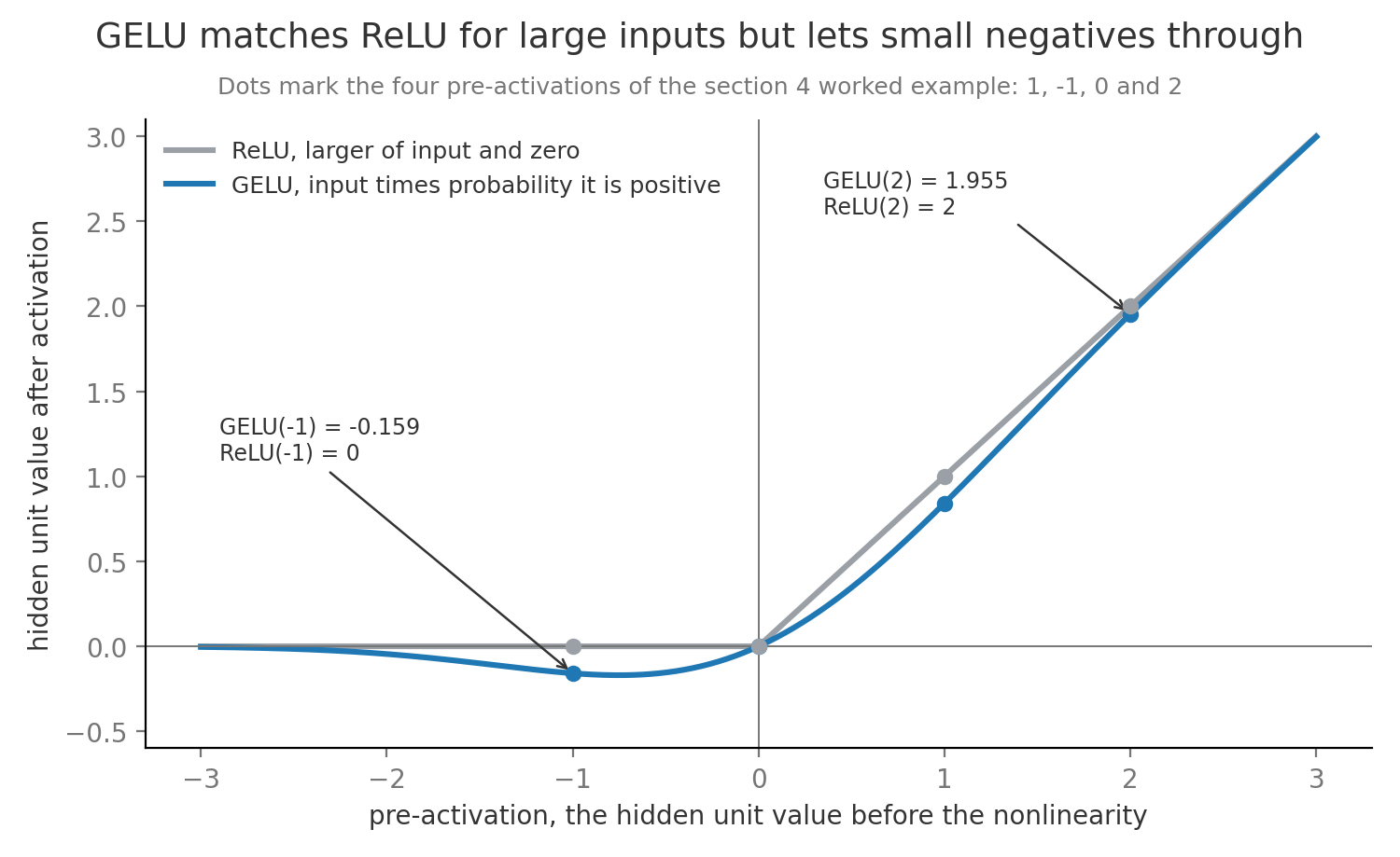
The activation is what makes the network more than one matrix, because two matrices in a row with nothing between them collapse into a single matrix. ReLU, the rectified linear unit, returns the larger of its input and zero. GELU, the Gaussian error linear unit from Hendrycks and Gimpel, returns for an input , where is the probability that a standard normal value falls below , so it behaves like ReLU for large inputs and lets small negative inputs through as small negative outputs. GPT-2 and BERT use GELU.
A feed-forward pass on a two-number token
Section titled “A feed-forward pass on a two-number token”The steps below push one two-number token through a feed-forward network with a hidden width of four, once with ReLU and once with GELU, so every multiplication can be checked.
- Use width and hidden width , and let the token be .
- Take the four columns of as , , , and . Each hidden unit is a dot product of with one column, meaning matching entries are multiplied and summed, giving pre-activations , , , and .
- ReLU turns these into . GELU gives , since , , and .
- Take the four rows of as , , , and . The output is each hidden value times its row, summed. With ReLU the output is . With GELU it is , which is the sublayer’s output that the block adds to the stream.
One useful reading from Geva et al. treats each column of as a key that detects a pattern in the input and the matching row of as the value written to the stream when that pattern fires. In step 4 the fourth hidden unit fired strongly and wrote twice. That reading explains why factual knowledge edits often target FFN weights, though most units respond to mixtures of patterns rather than one clean fact.
5. Gated activations and SwiGLU
Section titled “5. Gated activations and SwiGLU”A plain activation decides how much of each hidden unit passes based only on that unit’s own value. A gate lets a second learned signal make that decision, much as a mixing desk has a separate fader for each channel instead of letting the channel’s own volume decide. A gated linear unit, from Dauphin et al., computes two projections of the input and multiplies them, one acting as the gate and the other as the value. SiLU, the sigmoid linear unit, is , a smooth curve close to GELU. SwiGLU uses SiLU on the gate branch, as proposed by Shazeer:
Here and are both and produce the gate and the value, multiplies them coordinate by coordinate, and is and narrows the result back to width . Take a token whose gate pre-activations are and whose values are . SiLU gives and , so the gated hidden vector is . The first unit passes its value scaled up by 1.76, while the second shrinks its value to about a quarter and flips its sign, and the gate learned to make each call from the input.
Three matrices instead of two would raise the feed-forward network’s (FFN’s) parameters by half at the same hidden width, so the width is cut to keep the count near the classic . Setting gives , which is the source of the rule. For that is , rounded to 10,923, and Llama rounds up to the next multiple of 256 so the matrices split evenly across hardware tiles, giving . The SwiGLU FFN then holds parameters, 0.8% above . Shazeer’s experiments found the gated variants beat ReLU and GELU at matched parameters and compute, and PaLM, Llama, and Mistral all adopted SwiGLU. The paper offers no theory for why, so the usual explanation that multiplicative gates let a unit switch on context is a plausible reading rather than a proof.
6. The decoder block
Section titled “6. The decoder block”Sections 1 to 5 supply every part of a block, and assembling them is a matter of order, the way a workstation on an assembly line always performs the same two steps in the same sequence. A decoder block is the repeating unit of a text generator: a pre-norm attention sublayer followed by a pre-norm SwiGLU sublayer, each wrapped in a residual connection. For the attention sublayer it is enough here to know that multi-head attention splits the width into heads of width , and each head scores every earlier token, turns the scores into weights that sum to 1, and returns a weighted average of their information. The causal mask that makes it look only backward, and positional information, are developed in Attention and Positional Information. One block then computes
Here is the stream entering the block, is the stream after the attention sublayer has added its output, and is the stream leaving. Each RMSNorm has its own gain. The reference 7B stacks 32 identical copies, each with its own weights, and the input and output of every block are vectors of numbers per token.
flowchart TB X["Residual stream in<br/>width 4,096"] --> AT["RMSNorm 1, then<br/>multi-head attention<br/>32 heads of width 128"] AT --> P1(("+")) X -->|"identity path"| P1 P1 --> FF["RMSNorm 2, then<br/>SwiGLU feed-forward<br/>4,096 to 11,008 to 4,096"] FF --> P2(("+")) P1 -->|"identity path"| P2 P2 -->|"next block, or out<br/>after block 32"| OH["Final RMSNorm<br/>and output head<br/>32,000 logits, softmax"]The diagram shows why the two sublayers do different jobs. Attention is the only place tokens exchange information, so a block without it would process each word in isolation. The feed-forward network (FFN) is where most of the per-token computation and most of the parameters sit. Width stays at 4,096 on every edge of the identity path, which is what lets blocks be stacked, removed, or inspected one at a time. Llama 2 uses exactly this block, and the full list of later variants such as grouped-query attention and different position schemes is in Modern LLM Architectures.
7. The output head
Section titled “7. The output head”After the last block, the model has one 4,096-number vector per position and needs a probability for every possible next token. A quiz show contestant with a hunch must still say how confident they are in each answer on the board. The output head is one matrix of shape that turns the final normalized vector into one score per vocabulary entry. Each score is a logit, an unnormalized number where higher means more likely. Softmax then exponentiates every logit and divides by the total, producing probabilities that are positive and sum to 1:
Here is the stream after the last block, is the row of logits, is the logit for token , and the sum runs over the whole vocabulary of tokens. Take a three-token vocabulary of “cat”, “dog”, and “the”, a final normalized vector , and output columns , , and . The logits are , , and . Exponentials are 7.389, 2.718, and 1.105, which sum to 11.212, so the probabilities are 0.659, 0.242, and 0.099. If the true next token is “cat”, the training loss for this position is , and Language Modeling and Next Token Prediction develops that cross-entropy loss and the softmax in full.
Weight tying reuses the embedding table as the output matrix, since both map between tokens and -number vectors. It saves parameters, which is 131,072,000 in the reference 7B, only 1.9% of the model, so Llama 2 keeps them separate. In GPT-2 small, with and , the same table is 38.6 million of about 124 million parameters, roughly 31%, which is why small models usually tie. The head’s arithmetic is million operations per token, under 2% of the forward pass computed in section 9.
8. Parameter counting
Section titled “8. Parameter counting”Counting parameters is bookkeeping over matrix shapes, the same way a parts list for a bookshelf adds up boards by their dimensions. A matrix with 4,096 rows and 11,008 columns holds their product, 45,088,768 numbers, and the model’s total is the sum over every matrix and every normalization gain. The reference 7B, with blocks, width , vocabulary , and SwiGLU hidden width , counts as follows.
- Input embedding, one row per vocabulary entry: .
- Attention in one block, four matrices for queries, keys, values, and output: .
- SwiGLU FFN in one block, three matrices of : .
- Two RMSNorm gains in one block: . One block totals .
- All 32 blocks come to , the final RMSNorm adds 4,096, and the untied output head adds another 131,072,000.
- Total: , about 6.74 billion. At 2 bytes per number in bf16, a 16-bit number format, the weights take 13.48 GB, or 12.55 GiB in binary gigabytes of bytes.
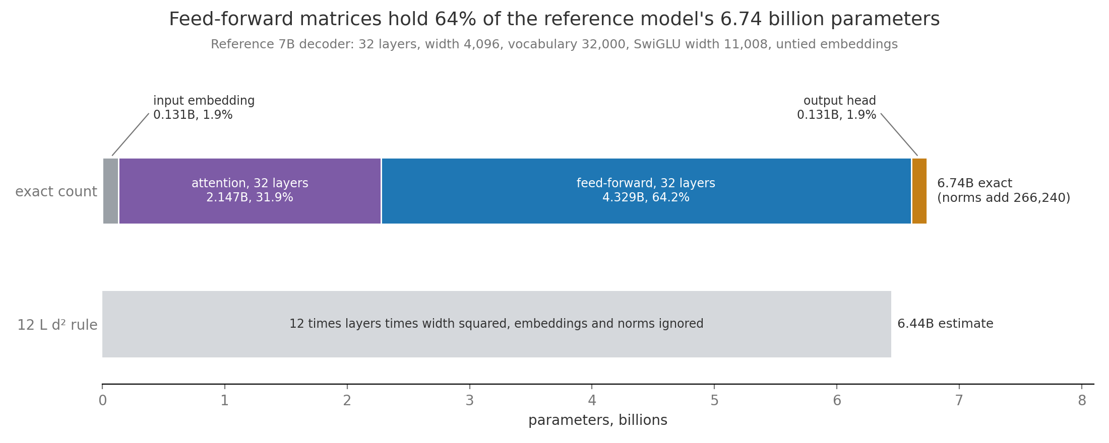
A quick estimate drops embeddings and norms and uses for attention plus for the feed-forward network (FFN), giving . For the reference model that is , about 4.4% below the exact count. Of that gap, 262 million is the two embedding tables and 33.5 million is SwiGLU’s rounding from 10,923 to 11,008. The estimate works well for large models and badly for small ones, where embeddings are a big share, as the GPT-2 small example in section 7 showed. Two common changes break the attention term. Grouped-query attention, where groups of query heads share one key head and one value head, shrinks the key and value matrices with 8 such groups to each, and a mixture of experts multiplies the FFN term, as section 10 shows.
9. FLOPs per token
Section titled “9. FLOPs per token”Parameter count says how much memory the weights need, and a separate count says how much arithmetic each token costs. A FLOP, or floating-point operation, is one addition or multiplication on a decimal number. Multiplying a token’s vector by a matrix takes multiplications and about additions, so every weight is used for about 2 FLOPs per token. The forward pass, computing the output from the input, therefore costs about FLOPs per token, where is the parameter count. For the reference 7B that is GFLOPs, where one GFLOP is a billion FLOPs.
The backward pass computes gradients and costs about twice the forward pass. For each matrix multiplication it needs two more of the same size, one giving the gradient for the layer’s input so the signal can continue to earlier layers and one giving the gradient for the weights so they can be updated. Training per token is therefore , which is 40.4 GFLOPs per token for the reference model. Over a training run of tokens this becomes the rule, FLOPs for 2 trillion tokens, which Pretraining at Scale turns into days on graphics processors. Recomputing intermediate results during the backward pass instead of storing them, which saves memory, adds roughly one more forward pass, about , so real runs often count more.
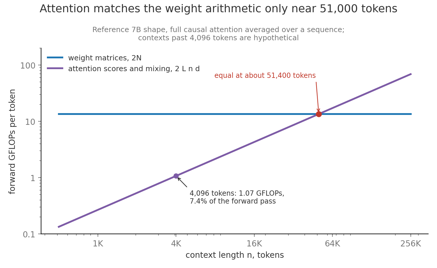
The rule leaves out attention’s own arithmetic, which has no weights. A token at position compares its query with keys and averages values, about FLOPs per block across all heads. Averaged over a causal sequence of context length , the number of tokens the model reads at once, this adds about per token. At that is GFLOPs, 7.4% of the forward pass. The two terms are equal when tokens, so for this shape the weights dominate until contexts get long, and attention then grows linearly per token while the weight term stays fixed. FLOPs set the cost of training and of processing a long prompt, but generating one token at a time is usually limited by reading the 13.48 GB of weights from memory instead, which Inference and Decoding works through.
10. Mixture of experts
Section titled “10. Mixture of experts”A dense model runs every parameter for every token, so making it know more also makes every token cost more. A hospital does not send each patient to every specialist, and a triage nurse picks two who fit the case. A mixture of experts, or MoE, applies the same idea to the feed-forward network (FFN), following Shazeer et al. and Switch Transformer. Each MoE layer keeps separate FFNs, each called an expert, and a router, a small learned matrix, scores the experts for each token. Top-k routing keeps the highest-scoring experts, renormalizes their router probabilities to sum to 1, and returns the weighted sum of their outputs. Attention, norms, and embeddings stay shared.
Routing one token through four experts
Section titled “Routing one token through four experts”The steps below route one token through a layer of four experts that keeps the top two, from the router scores to the weighted output.
- Take experts, , and router scores for one token.
- Softmax gives probabilities , so the top two are experts 1 and 2.
- Renormalizing the kept pair gives and . If expert 1 returns and expert 2 returns , the layer outputs . Experts 3 and 4 do no arithmetic for this token.
The animation then routes five more tokens. Six tokens make 12 assignments, a fair share of 3 per expert, but expert 2 receives 5 and expert 4 only 1. Left alone this worsens, because a busier expert trains faster and attracts still more tokens, until a few experts take everything. A load balancing loss, an extra training penalty that grows when assignments are uneven, keeps the experts in use, and Advanced Topics derives it along with the capacity limits that drop overflow tokens.
The payoff and the cost show up in two counts. Total parameters are every weight stored, which sets memory. Active parameters are the weights one token actually multiplies against, which sets FLOPs. Replace the reference 7B’s FFN with 8 SwiGLU experts of the same size and route top-2. Each expert holds 135,266,304 parameters, and the router adds per block. Total parameters become 37.04 billion, which is 74.1 GB in bf16, while active parameters are 11.07 billion, so each token costs about GFLOPs forward. The model stores 5.5 times the dense model’s weights for 1.6 times its arithmetic. Mixtral 8x7B, from Jiang et al., has 46.7 billion total and 12.9 billion active, and Modern LLM Architectures covers how much quality the extra storage actually buys, which is less than the storage ratio.
11. Architecture families and training objectives
Section titled “11. Architecture families and training objectives”The same blocks can be wired three ways, and the wiring decides what the model can be trained to do. A reader who sees a whole sentence with blanks to fill learns something different from a writer who only ever sees the words so far. Each family pairs an attention pattern with an objective, the prediction task whose error training minimizes. An encoder-only model such as BERT lets every token see every other token and trains with masked language modeling, hiding about 15% of tokens and predicting them. A decoder-only model such as GPT or Llama uses a causal mask so each token sees only earlier ones, and trains with causal language modeling, predicting the next token at every position. An encoder-decoder model such as T5 reads a source with a bidirectional encoder and writes the output with a causal decoder that also uses cross attention, attention whose queries come from the output and whose keys and values come from the encoded source. T5 trains with span corruption, replacing random runs of tokens with placeholder markers and generating the missing runs. A prefix LM, or prefix language model, is a decoder-only model whose first part, the prefix, is read bidirectionally while the rest is generated causally.
The objectives differ sharply in how much signal one sequence gives. In a 512-token sequence, masked modeling yields about predictions, while causal modeling yields about 512, one per position. T5’s span corruption with spans averaging 3 tokens yields the same 77 hidden tokens in about 26 spans. Decoder-only models came to dominate general-purpose large language models for four connected reasons. They extract a learning signal from every token. One objective serves every task through prompting, since any task can be written as text to continue. Generation streams naturally one token at a time while reusing stored results for earlier tokens. With a single stack there are fewer design choices to scale. Wang et al. found causal decoders best for zero-shot use, meaning tasks given without examples, after plain pretraining on raw text, while encoder-decoders did better after multitask fine-tuning, meaning further training on many labeled tasks, so the win is about the general-purpose use case rather than every task.
| Situation | Choice | Main qualification |
|---|---|---|
| General assistant, open-ended generation, prompting with a few examples | Dense decoder-only | Cost per token grows with every parameter |
| Embeddings, retrieval, or classification at low latency | Encoder-only | Cannot generate text |
| Fixed input mapped to a different output, such as translation or speech | Encoder-decoder | Two stacks to scale and serve |
| Quality per FLOP matters and memory across many graphics processors is available | Decoder-only mixture of experts | Memory follows total parameters and needs load balancing |
| One graphics processor or an edge device with tight memory | Small dense decoder-only | Lower ceiling on quality |
At staff level the choice between a dense model and a mixture of experts gets decided by an experiment with a stated exit. Fix a training budget in FLOPs, train both at that budget on the same data, and compare quality alongside serving cost per million tokens at the expected batch size. Write the reversal condition down before the run, for instance that the dense model ships if serving memory or the communication between graphics processors holding different experts makes the mixture’s cost per token higher at equal quality.
Related: Language Modeling and Next Token Prediction · Tokenization and Embeddings · Attention and Positional Information · Pretraining at Scale · Inference and Decoding